Setting up and Managing Storage Devices

The storage infrastructure supporting VMware has always been a critical element of any virtual infrastructure. This chapter will help you with all the elements required for a proper storage subsystem design for vSphere 4, starting with VMware storage fundamentals at the datastore and virtual machine level and extending to best practices for configuring the storage array. Good storage design is critical for anyone building a virtual datacenter.

Why storage design is important?

Storage design has always been important, but it becomes more so as vSphere is used for larger workloads, for mission-critical applications, for larger clusters, and as the cloud operating system in a 100 percent virtualized datacenter. You can probably imagine why this is the case:

Advanced capabilities VMware's advanced features depend on shared storage; VMware High Availability (HA), VMotion, VMware Distributed Resource Scheduler (DRS), VMware Fault Tolerance, and VMware Site Recovery Manager all have a critical dependency on shared storage.

Performance People understand the benefit that server virtualization brings-consolidation, higher utilization, more flexibility, and higher efficiency. But often, people have initial questions about how vSphere can deliver performance for individual applications when it is inherently consolidated and oversubscribed. Likewise, the overall performance of the virtual machines and the entire vSphere cluster are both dependent on shared storage, which is similarly inherently highly consolidated, and oversubscribed.

Availability The overall availability of the virtual machines and the entire vSphere cluster are both dependent on the shared storage infrastructure. Designing in high availability into this infrastructure element is paramount. If the storage is not available, VMware HA will not be able to recover, and the aggregate community of VMs on the entire cluster can be affected.

Whereas there are design choices at the server layer that can make the vSphere environment relatively more or less optimal, the design choices for shared resources such as networking and storage can make the difference between virtualization success and failure. This is regardless of whether you are using storage area networks (SANs), which present shared storage as disks or logical units (LUNs), or whether you are using network attached storage (NAS), which presents shared storage as remotely accessed file systems or a mix of both. Done correctly, a shared storage design lowers the cost and increases the efficiency, performance, availability, and flexibility of your vSphere environment.

Shared Storage Fundamentals

vSphere 4 significantly extends the storage choices and configuration options relative to VMware Infrastructure 3.x. These choices and configuration options apply at two fundamental levels: the ESX host level and the virtual machine level. The storage requirements for each vSphere cluster and he virtual machines it supports are uniquemaking broad generalizations impossible. The requirements for any given cluster span use cases, from virtual servers to desktops to templates and (ISO) images. The virtual server use cases that vary from light utility VMs with few storage performance considerations to the largest database workloads possible wih incredibly important storage layout considerations.

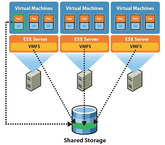
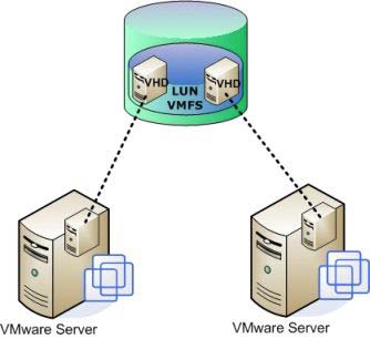
Let's start by examining this at a fundamental level. Figure 6.1 shows a simple three-host vSphere 4 cluster attached to shared storage.

It's immediately apparent that the vSphere ESX 4 hosts and the virtual machines will be contending for the shared storage asset. In an analogous way to how vSphere ESX 4 can consolidate many virtual machines onto a single host, the shared storage consolidates all the storage needs of all the virtual machines.

What are the implications of this? The virtual machines will depend on and share the performance characteristics of the underlying storage configuration that supports them. Storage attributes are just as important as CPU cycles (measured in megahertz), memory (measured in megabytes), and vCPU configuration. Storage attributes are measured in capacity (gigabytes) and performance, which is measured in bandwidth (MB per second or MBps), throughput (1/0 per second or lOps), and latency (in milliseconds).

The overall availability of the virtual machines and the entire vSphere cluster is dependent on the same shared storage infrastructure so a robust, design is paramount. If the storage is not available, VMware HA will not be able to recover, and the consolidated community of VMs will be affected. One critical premise of storage design is that more care and focus should be put on the availability of the configuration than on the performance or capacity requirements:

• With advanced vSphere options such as Storage VMotion and advanced array techniques that allow you to add, move, or change storage configurations non disruptively, it is unlikely that you'll create a design where you can't non disruptively fix performance Issues.

• Conversely, in virtual configurations, the availability impact of storage issues is more pronounced, so greater care needs to be used in an availability design than in the physical world.

An ESX server can have one or more storage options actively configured, including the following:

Fibre Channel

• Fibre Channel over Ethernet

• iSCSI using software and hardware initiators

• NAS (specifically, NFS)

• Local SAS/SATA/SCSI storage

• InfiniBand

Shared storage is the basis for most of VMware storage because it supports the virtual machines themselves. Shared storage in both SAN configurations (which encompasses Fibre Channel, iSCSI, FCoE) and NAS is always highly consolidated. This makes it very efficient. In an analogous way that VMware can take many servers with 10 percent utilized CPU and memory and consolidate them to make them 80 percent utilized, SAN/NAS takes the direct attached storage in servers that are 10 percent utilized and consolidates them to 80 percent utilization. Local storage is used in a limited fashion with VMware in general, and local storage in vSphere serves even less of a function than it did in VMware Infrastructure 3.x because it is easier to build and add hosts using ESX host profiles.

How carefully does one need to design their local storage? The answer is simple-careful planning is not necessary for storage local to the vSphere ESX/ESXi host. vSphere ESX/ESXi 4 stores very little locally, and by using host profiles and distributed virtual switches, it can be easy and fast to replace a failed ESX host. During this time, VMware HA will make sure the virtual machines are running on the other ESX hosts in the cluster. Don't sweat; HA design in local storage for ESX. Spend the effort making your shared storage design robust.

Local storage is still used by default in vSphere ESX 4 installations as the ESX userworld swap (think of this as the ESX host swap and temp use), but not for much else. Unlike ESX 3.x, where VMFS mounts on local storage are used by the Service Console, in ESX 4, although there is a Service Console, it is functionally a virtual machine using a virtual disk on the local VMFS storage.

Before going too much further, it's important to cover several basics of shared storage:

• Common storage array architectures

• RAID technologies

• Midrange and enterprise storage design

• Protocol choices

The high-level overview in the following sections is neutral on specific storage array vendors, because the internal architectures vary tremendously. However, these sections will serve as an important baseline for the discussion of how to apply these technologies as well as the analysis of new technologies.

Common Storage Array Architectures

This section is remedial for anyone with basic storage experience but is needed for VMware administrators with no preexisting storage knowledge. For people unfamiliar with storage, the topic can be a bit disorienting at first. Servers across vendors tend to be relatively similar, but the same logic can't be applied to the storage layer, because core architectural differences are vast between storage vendor architectures. In spite of that, storage arrays have several core architectural elements that are consistent across vendors, across implementations, and even across protocols.

The elements that make up a shared storage array consist of external connectivity, storage processors, array software, cache memory, disks, and bandwidth: External connectivity The external (physical) connectivity between the storage array and the hosts (in this case, the VMware ESX 4 servers) is generally Fibre Channel or Ethernet, though InfiniBand and other rare protocols exist. The characteristics of this connectivity define the maximum bandwidth (given no other constraints, and there usually are other constraints) of the communication between the host and the shared storage array.

Storage processors Different vendors have different names for storage processors, which are considered the "brains" of the array. They are used to handle the I/O and run the array software.

In most modem arrays, the storage processors are not purpose-built ASICs but instead are general-purpose CPUs. Some arrays use PowerPC, some use specific ASICs, and some use custom ASICs for specific purposes. But in general, if you cracked open an array, you would most likely find an Intel or AMD CPU.

Array software Although hardware specifications are important and can define the scaling limits of the array, just as important are the functional capabilities the array software provides. The array software is at least as important as the array hardware. The capabilities of modern storage arrays are vast-similar in scope to vSphere itself-and vary wildly between vendors.

At a high level, the following list includes some examples of these array capabilities; this is not an exhaustive list but does include the key functions:

• Remote storage replication for disaster recovery. These technologies come in many flavors with features that deliver varying capabilities. These include varying recovery point objectives (RPOs)-which is a reflection of how current the remote replica is at any time ranging from synchronous, to asynchronous and continuous. Asynchronous RPOs can range from minutes to hours, and continuous is a constant remote journal which can recover to varying Recovery Point Objectives. Other examples of remote replication technologies are technologies that drive synchronicity across storage objects or "consistency technology," compression, and many other attributes such as integration with VMware Site Recovery Manager.

• Snapshot and clone capabilities for instant point-in-time local copies for test and development and local recovery. These also share some of the ideas of the remote replication technologies like "consistency technology" and some variations of point-in-time protection and replicas also have "TiVo-like" continuous journaling locally and remotely where you can recovery / copy any point in time.

• Capacity reduction techniques such as archiving and deduplication.

• Automated data movement between performance/cost storage tiers at varying levels of granularity.

• LUN/file system expansion and mobility, which means reconfiguring storage properties dynamically and non-disruptively to add capacity or performance as needed.

• Thin provisioning. #

• Storage quality of service, which means prioritizing I/O to deliver a given MBps, lOps, or latency.

The array software defines the "persona" of the array, which in turn impacts core concepts and behavior in a variety of ways. Arrays generally have a "file server" persona (sometimes with the ability to do some block storage by presenting a file as a LUN) or a "block" persona (generally with no ability to act as a file server). In some cases, arrays are combinations of file servers and block devices put together.

Cache memory Every array differs on how this is implemented, but all have some degree of nonvolatile memory used for various caching functions-delivering lower latency and higher laps throughput by buffering I/O using write caches and storing commonly read data to deliver a faster response time using read caches. NonvolatiJity (meaning it survives a power loss) is critical for write cache because the data is not yet committed to disk, but it's not critical for read caches. Cached performance is often used when describing shared storage array performance maximums (in lOps, MBps, or latency) in specification sheets. These results are generally not reflective of real-world scenarios. In most real-world scenarios, performance tends to be dominated by the disk performance (the type and amount of disks) and is helped by write cache in most cases but only marginally by read caches (with the exception of large Relational Database Management Systems, which depend heavily on read-ahead cache algorithms). One VMware use case that is helped by read caches can be cases where many boot images are stored only once (through use of VMware or storage array technology), but this is also a small subset of the overall virtual machine 10 pattern.

Disks Arrays differ on which type of disks (often called spindles) they support and how many they can scale to support. Fibre Channel (usually in 15KB RPM and lOKB RPM variants), SATA (usually in 5400 RPM and 7200 RPM variants), and SAS (usually in 15K RPM and 10K RPM variants) are commonplace, and enterprise flash disks are becoming mainstream. The type of disks and the number of disks are very important. Coupled with how they are configured, this is usually the main determinant of how a storage object (either a LUN for a block device or a file system for a NAS device) performs. Shared storage vendors generally use disks from the same disk vendors, so this is an area where there is commonality across shared storage vendors.

The following list is a quick reference on what to expect under a random read/write workload from a given disk drive:

• 7200RPM SATA: 80 lOps

• lOKB RPM SATA/SAS/Fibre Channel: 120 lOps

• 15KB RPM SAS/Fibre Channel: 180 laps

• A commercial solid-state drive (SSD) based on Multi-Layer Cell (MLC) technology:

• 1000-2000 laps

• An Enterprise Flash Drive (EFD) based on single-layer cell (SLC) technology and much deeper, very high-speed memory buffers: 6000-30,000 lOps

Bandwidth (megabytes per second) Performance tends to be more consistent across drive types when large-block, sequential workloads are used (such as single-purpose workloads like archiving or backup to disk), so in these cases, large SATA drives deliver strong performance at a low cost.

RAID Technologies

Redundant Array of Inexpensive (sometimes "independent") Disks (RAID) is a fundamental, but critical, method of storing the same data several times, and in different ways to increase the data availability, and also scale performance beyond that of a single drive., Every array implements various RAID schemes (even if it is largely "invisible" in file server persona arrays where

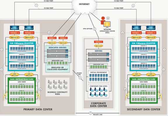
HIGH AVAILABILITY HOSTED VMware INFRASTRUCTURE SOLUTIONS

RAID is done below the primary management element which is the filesystem).

Think of it this way: "disks are mechanical spinning rust-colored disc surfaces. The read/write heads are flying microns above the surface. While they are doing this, they read minute magnetic field variations, and using similar magnetic fields, write data by affecting surface areas also only microns in size."

Remember, all the RAID protection in the world won't protect you from an outage if the connectivity to your host is lost, if you don't monitor and replace failed drives and allocate drives as hot spares to automatically replace failed drives, or if the entire array is lost. It's for these reasons that it's important to design the storage network properly, to configure hot spares as advised by the storage vendor, and monitor for and replace failed elements. Always consider a disaster recovery plan and remote replication to protect from complete array failure. Let's examine the RAID choices:

RAID0 - This RAID level offers no redundancy and no protection against drive failure (see Figure 6.2). In fact, it has a higher aggregate risk than a single disk because any single disk failing affects the whole RAID group. Data is spread across all the disks in the RAID group, which is often called a stripe. Although it delivers very fast performance, this is the only RAID type that is not appropriate for any production VMware use, because of the availability profile.

RAID 1, 1+0, 0+1 These "mirrored" RAID levels offer high degrees of protection but at the cost of 50 percent loss of usable capacity (see Figure 6.3). This is versus the raw aggregate capacity of the sum of the capacity of the drives. RAID 1 simply writes every I/O to two drives and can balance reads across both drives (since there are two copies). This can be coupled with RAID 0 or with RAID 1+0 (or RAID 10), which mirrors a stripe set, and with RAID 0+1, which stripes data across pairs of mirrors. This has the benefit of being able to withstand multiple drives failing, but only if the drives fail on different elements of a stripe on different mirrors.

The other benefit of mirrored RAID configurations is that, in the case of a failed drive, rebuild times can be very rapid, which shortens periods of exposure.

Parity RAID (RAID 5, RAID 6) These RAID levels use a mathematical calculation (an XOR parity calculation) to represent the data across several drives. This tends to be a good compromise between the availability of RAID 1 and the capacity efficiency of RAID O. RAID 5 calculates the parity across the drives in the set and writes the parity to another drive. This parity block calculation with RAID 5 is rotated amongst the arrays in the RAID 5 set. (RAID 4 is a variant that uses a dedicated parity disk rather than rotating the parity across drives.)Parity RAID schemes can deliver very good performance. There is always some degree of "write penalty." For a full-stripe write, the only penalty is the parity calculation and the parity write, but in a partial-stripe write, the old block contents need to be read, a new parity calculation needs to be made, and all the blocks need to be updated. However, generally modern arrays have various methods to minimize this effect.

Conversely, read performance is excellent, because a larger number of drives can be read from than with mirrored RAID schemes. RAID 5 nomenclature refers to the number of drives in the RAID group.

When a drive fails in a RAID 5 set, I/Os can be fulfilled using the remaining drives and the parity drive, and when the failed drive is replaced, the data can be reconstructed using the remaining data and parity.

This last type of RAID is called RAID 6 (RAID-DP is a RAID 6 variant that uses two dedicated parity drives, analogous to RAID 4). This is a good choice when very large RAID groups and SATA are used.

Take an example of a RAID 6 4+2 configuration. The data is striped across four disks, and a parity calculation is stored on the fifth disk. A second parity calculation is stored on another disk. RAID 6 rotates the parity location with I/O, and RAID-DP uses a pair of dedicated parity disks. This provides good performance and good availability but a loss in capacity efficiency. The purpose of the second parity bit is to withstand a second drive failure during RAID rebuild periods. It is important to use RAID 6 in place of RAID 5 if you meet the conditions noted in the "A Key RAID 5 Consideration" section and are unable to otherwise use the mitigation methods noted.

Protocol Choices

VMware vSphere 4 offers several shared protocol choices, ranging from Fibre Channel, iSCSI, FCoE, and Network File System (NFS), which is a form of NAS. A little understanding of each goes a long way in designing your VMware vSphere environment.

Fibre channel

SANs are most commonly associated with Fibre Channel storage, because Fibre Channel was the first protocol type used with SANs. However, SAN refers to a network topology, not a connection protocol. Although often people use the acronym SAN to refer to a Fibre Channel SAN, it is completely possible to create a SAN topology using different types of protocols, including iSCSI, FCoE and InfiniBand. SANs were initially deployed to mimic the characteristics of local or direct attached SCSI devices. A SAN is a network where storage devices (Logical Units-or LUNs-just like on a SCSI or SAS controller) are presented from a storage target (one or more ports on an array) to one or more initiators. An initiator is usually a host bus adapter (HBA), though software-based initiators are also possible for iSCSI and FCoE.

Today, Fibre Channel HBAs have roughly the same cost as high-end multiported Ethernet interfaces or local SAS controllers, and the per-port cost of a Fibre Channel switch is about twice that of a high-end managed Ethernet switch.

Fibre Channel uses an optical interconnect (though there are copper variants), which is used since the Fibre Channel protocol assumes a very high-bandwidth, low-latency, and lossless physical layer. Standard Fibre Channel HBAs today support very high-throughput, 4Gbps and 8Gbps, connectivity in single-, dual-, and even quad-ported options. Older, obsolete HBAs supported only 2Gbps. Some HBAs supported by vSphere ESX 4 are the QLogic QLE2462 and Emulex LPlOOOO.

The Fibre Channel protocol can operate in three modes: point-to-point (FC-P2P), arbitrated loop (FC-AL), and switched (FC-SW). Point-to-point and arbitrated loop are rarely used today for host connectivity, and they generally predate the existence of Fibre Channel switches. FC-AL is commonly used by some array architectures to connect their "back-end spindle enclosures" (vendors call these different things, but they're the hardware element that contains and supports the physical disks) to the storage processors, but even in these cases, most modern array designs are moving to switched designs, which have higher bandwidth per disk enclosure.

iSCSI

iSCSI brings the idea of a block storage SAN to customers with no Fibre Channel infrastructure. iSCSI is an IETF standard for encapsulating SCSI control and data in TCPlIP packets, which in tum are encapsulated in Ethernet frames. Figure 6.13 shows how iSCSI is encapsulated in TCP/ IP and Ethernet frames. TCP retransmission is used to handle dropped Ethernet frames or significant transmission errors. Storage traffic can be intense relative to most LAN traffic. This makes minimizing retransmits, minimizing dropped frames, and ensuring that you have "bet-the-business" Ethernet infrastructure important when using iSCSI.

Although often Fibre Channel is viewed as higher performance than iSCSI, in many cases iSCSI can more than meet the requirements for many customers, and carefully planned and scaled-up iSCSI infrastructure can, for the most part, match the performance of a moderate Fibre ChannelSAN.

Also, the overall complexity of iSCSI and Fibre Channel SANs are roughly comparable and share many of the same core concepts. Arguably, getting the first iSCSI LUN visible to a vSphere ESX host is simpler than getting the first Fibre Channel LUN visible for people with expertise with Ethernet but not Fibre Channel, since understanding worldwide names and zoning is not needed. However, as you saw earlier, these are not complex topics. In practice, designing a scalable, robust iSCSI network requires the same degree of diligence that is applied to Fibre Channel; you should use VLAN (or physical) isolation techniques similarly to Fibre Channel zoning and need to scale up connections to achieve comparable bandwidth.

Each ESX host has a minimum of two VMkernel ports, and each is physically connected to two Ethernet switches. Storage and LAN are isolated-physically or via VLANs. Each switch has a minimum of two connections to two redundant front-end array network interfaces (across storage processors) .

Also, when examining iSCSI and iSCSI SANs, many core ideas are similar to Fibre Channel and Fibre Channel SANs, but in some cases there are material differences. Let's look at the terminology:

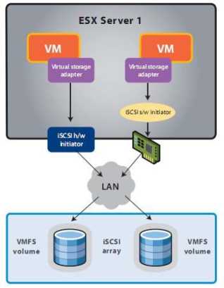
iSCSI initiator An iSCSI initiator is a logical host-side device that serves the same function as a physical host bus adapter in Fibre Channel or SCSI/SAS. iSCSI initiators can be software initiators (which use host CPU cycles to load/unload SCSI payloads into standard TCP/IP packets and perform error checking). Examples of software initiators that are pertinent to VMware administrators are the native vSphere ESX software initiator and the guest software initiators available in Windows XP and later and in most current Linux distributions. The other form of iSCSI initiators are hardware initiators. These are QLogic QLA 405x and QLE 406x host bus adapters that perform all the iSCSI functions in hardware. An iSCSI initiator is identified by an iSCSI qualified name. An iSCSI initiator uses an iSCSI network portal that consists of one or more IP addresses. An iSCSI initiator "logs in" to an iSCSI target.

iSCSI target An iSCSI target is a logical target-side device that serves the same function as a target in Fibre Channel SANs. It is the device that hosts iSCSI LUNs and masks to specific iSCSI initiators. Different arrays use iSCSI targets differently-some use hardware, some use software implementations-but largely this is unimportant. More important is that an iSCSI target doesn't necessarily map to a physical port as is the case with Fibre Channel; each array does this differently. Some have one iSCSI target per physical Ethernet port; some have one iSCSI target per iSCSI LUN, which is visible across multiple physical ports; and some have logical iSCSI targets that map to physical ports and LUNs in any relationship the administrator configures within the array. An

iSCSI target is identified by an iSCSI Qualified Name. An iSCSI target uses an iSCSI

network portal that consists of one or more IP addresses.

• iSCSI Logical Unit (LUN) An iSCSI LUN is a LUN hosted by an iSCSI target.

There can be one or more LUNs "behind" a single iSCSI target.

• iSCSI network portal An iSCSI network portal is one or more IP addresses that are used by an iSCSI initiator or iSCSI target.

• iSCSI Qualified Name (IQN) An iSCSI qualified name (IQN) serves the purpose of the WWN in Fibre Channel SANs; it is the unique identifier for an iSCSI initiator, target, or LUN. The format of the IQN is based on the iSCSI IETF standard.

• Challenge Authentication Protocol (CHAP) CHAP is a widely used basic authentication protocol, where a password exchange is used to authenticate the source or target of communication. Unidirectional CHAP is one-way; the source authenticates to the destination, or, in the case of iSCSI, the iSCSI initiator authenticates to the iSCSI target. Bidirectional CHAP is two-way; the iSCSI initiator authenticates to the iSCSI target, and vice versa, before communication is established. Although Fibre Channel SANs are viewed as "intrinsically" secure because they are physically isolated from the Ethernet network and although initiators not zoned to targets cannot communicate, this is not by definition true of iSCSI. With iSCSI, it is possible (but not recommended) to use the same Ethernet segment as general LAN traffic, and there is no intrinsic "zoning" model. Because the storage and general networking traffic could share networking infrastructure, CHAP is an optional mechanism to authenticate the source and destination of iSCSI traffic for some additional security. In practice, Fibre Channel and iSCSI SANs have the same security, and same degree of isolation (logical or physical).

• IP Security (IPsec) IPsec is an IETF standard that uses public-key encryption techniques to secure the iSCSI payloads so that they are not susceptible to man-in-the-middle security attacks. Like CHAP for authentication, this higher level of optional security is part of the iSCSI standards because it is possible (but not recommended) to use a general-purpose IP network for iSCSI transport-and in these cases, not encrypting data exposes a security risk (for example, a man-in-the-middle could determine data on a host they can't authenticate to by simply reconstructing the data from the iSCSI packets). IPsec is relatively rarely used, as it has a heavy CPU impact on the initiator and the target.

• Static/dynamic discovery iSCSI uses a method of discovery where the iSCSI initiator can query an iSCSI target for the available LUNs. Static discovery involves a manual configuration, whereas dynamic discovery issues an iSCSI-standard SendTargets command to one of the iSCSI targets on the array. This target then reports all the available targets and LUNs to that particular initiator. iSCSI Naming Service (iSNS) The iSCSI Naming Service is analogous to the Domain Name Service

(DNS); it's where an iSNS server stores all the available iSCSI targets for a very large iSCSI deployment. iSNS is relatively rarely used.

In general, the iSCSI session can be multiple TCP connections, called Multiple Connections Per Session." Note that this cannot be done in VMware. An iSCSI initiator and iSCSI target can communicate on an iSCSI network portal that can consist of one or more IP addresses. The concept of network portals is done differently on each array-some always having one IP address per target port, some using network portals extensively-there is no wrong or right, but they are different. The iSCSI initiator logs into the iSCSI target, creating an iSCSI session. It is possible to have many iSCSI sessions for a single target, and each session can potentially have multiple TCP connections (multiple connections per session). There can be varied numbers of iSCSI LUNs behind an iSCSI target-many or just one. Every array does this differently.

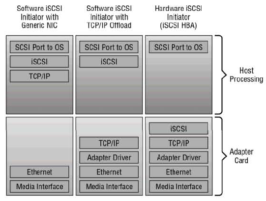
What about the furious debate about hardware iSCSI initiators (iSCSI HBAs) versus software iSCSI initiators? Figure 4.1 shows the difference between software iSCSI on generic network interfaces, those that do TCPIP offload, full iSCSI HBAs. Clearly there are more things the host (the ESX server) needs to process with software iSCSI initiators, but the additional CPU is relatively light.

Figure 4.1

Fully saturating several GbE links will use only roughly one core of a modern CPU, and the cost of iSCSI HBAs is usually less than the cost of slightly more CPU. More and more often-software iSCSI initiators are what the customer chooses.

NFS

The Network File System (NFS) protocol is a standard originally developed by Sun Microsystems to enable remote systems to be able to access a file system on another host as if it was locally attached. VMware vSphere (and ESX 3.x) implements a client compliant with NFSv3 using TCP.

When NFS datastores are used by VMware, no local file system (i.e., VMFS) is used. The file system is on the remote NFS server. This moves the elements of storage design related to supporting the file system from the ESX host to the NFS server; it also means that you don't need to handle zoning/masking tasks. This makes configuring an NFS datastore one of the easiest storage options to simply get up and running.

Technically, any NFS server that complies with NFSv3 over TCP will work with VMware, but similarly to the considerations for Fibre Channel and iSCSI, the infrastructure needs to support your entire VMware environment. As such, only use NFS servers that are explicitly on the VMwareHCL.

Using NFS datastores move the elements of storage design associated with LUNs from the ESX hosts to the NFS server. The NFS server has an internal block storage configuration, using some RAID levels and similar techniques discussed earlier, and create file systems on those block storage devices. With most enterprise NAS devices, this configuration is automated, and is done "under the covers." Those file systems are then exported via NFS and mounted on the ESX hosts in the cluster.

Beyond the IP storage considerations for iSCSI (which are similarly useful on NFS storage configurations), also consider the following:

• Consider using switches that support cross-stack EtherChannel. This can be useful in creating high-throughput, highly available configurations.

• Multipathing and load balancing for NFS use the networking stack of ESX, not the storage stack-so be prepared for careful configuration of the end-to-end network and NFS server configuration.

• Each NFS datastore uses two TCP sessions to the NFS server: one for NFS control traffic and the other for the data traffic. In effect, this means that the vast majority of the NFS traffic for a single datastore will use a single TCP session, which in turn means that link aggregation will use one Ethernet link per datastore. To be able to use the aggregate throughput of multiple Ethernet interfaces, multiple datastores are needed, and the expectation should be that no single datastore will be able to use more than one link's worth of bandwidth. The new approach available to iSCSI (multiple iSCSI sessions per iSCSI target) is not available in the NFS use case.

VMFS version 3 Datastores

The VMware File System (VMFS) is the most common configuration option for most VMware deployments. It's analogous (but different) to NTFS for Windows Server and ext3 for Linux. Like these file systems, it is native; it's included with vSphere and operates on top of block storage objects.

The purpose of VMFS is to simplify the storage environment in the VMware context. It would clearly be difficult to scale a virtual environment if each virtual machine directly accessed its own storage rather than storing the set of files on a shared volume. It creates a shared storage pool that is used for a set of virtual machines.

VMFS differs from these common file systems in several important fundamental ways:

It was designed to be a clustered file system from its inception, but unlike most clustered file systems, it is simple and easy to use. Most clustered file systems come with manuals the size of a phone book.

This simplicity is derived from its simple and transparent distributed locking mechanism.

This is generally much simpler than traditional clustered file systems with network cluster lock managers (the usual basis for the giant manuals).

It enables simple direct-to-disk, steady-state I/O that results in very high throughput at a very low CPU overhead for the ESX server.

Locking is handled using metadata in a hidden section of the file system. The metadata portion of the file system contains critical information in the form of on-disk lock structures (files) such as which vSphere 4 ESX server is the current owner of a given virtual machine, ensuring that there is no contention or corruption of the virtual machine

When these on-disk lock structures are updated, the ESX 4 host doing the update, which is the same mechanism that was used in ESX 3.x, momentarily locks the LUN using a nonpersistent SCSI lock (SCSI Reserve/Reset commands). This operation is completely transparent to the VMware administrator.

These metadata updates do not occur during normal I/O operations and are not a fundamental scaling limit.

During the metadata updates, there is minimal impact to the production I/O. This impact is negligible to the other hosts in the ESX cluster, and more pronounced on the host holding the SCSI lock.

These metadata updates occur during the following:

The creation of a file in the VMFS datastore (creating/deleting a VM, for example, or taking an ESX snapshot)

Actions that change the ESX host that "owns" a virtual machine (VMotion and VMwareHA)

The final stage of a Storage VMotion operation in ESX 3.5 (but not vSphere)

Change's to the' VMFS file' system itself (extending the file system or adding a file system extent) VMFS is currently at version 3 and does not get updated as part of the VMware Infrastructure 3.x to vSphere 4 upgrade process, one of many reasons why the process of upgrading from VI3.5 to vSphere can be relatively simple.

A VMFS file system exists on one or more partitions or extents. It can be extended by dynamically adding more extents; up to 32 extents are supported. There is also a 64TB maximum VMFS version 3 file system size. Note that individual files in the VMFS file system can span extents, but the maximum file size is determined by the VMFS allocation size during the volume creation, and the maximum remains 2TB with the largest allocation size selected. In prior versions of VMware ESX, adding a partition required an additional LUN, but in vSphere, VMFS file systems can be dynamically extended into additional space in an existing LUN.

The spanned VMFS includes two extents-the primary partition (in this case a 10GB LUN) and the additional partition (in this case a 100GBLUN). As files are created, they are spread around the extents, so although the volume isn't striped over the extents, the benefits of the increased performance and capacity are used almost immediately.

It is a widely held misconception that having a VMFS file system that spans multiple extents is always a bad idea and acts as a simple "concatenation" of the file system. In practice, although adding a VMFS extent adds more space to the file system as a concatenated space, as new objects (VMs) are placed in the file system, VMFS version 3 will randomly distribute those new file objects across the various extents-without waiting for the original extent to be full. VMFS version 3 (since the days of ESX 3.0) allocates the initial blocks for a new file randomly in the file system, and subsequent allocations for that file are sequential. This means that files are distributed across the file system and, in the case of spanned VMFS volumes, across multiple LUNs. This will naturally distribute virtual machines across multiple extents.

The Importance of LUN Queues

Queues are an important construct in block storage use cases (across all protocols, including iSCSI Fibre Channel, and FCoE). Think of a queue as a line at the supermarket checkout. Queues exist on the server (in this case the ESX server), generally at both the HBA and LUN levels. They also exist on the storage array. Every array does this differently, but they all have the same concept. Block-centric storage arrays generally have these queues at the target ports, array-wide, and array LUN levels, and finally at the spindles themselves. File-server centric designs generally have queues at the target ports, and array-wide, but abstract the array LUN queues as the LUNs exist actually as files in

the file system. However, fileserver centric designs have internal LUN queues underneath the file systems themselves, and then ultimately at the spindle level-in other words it's "internal" to how the file server accesses its own storage.

VMware Server

VMware Server

The queue depth is a function of how fast things are being loaded into the queue and how fast the queue is being drained. How fast the queue is being drained is a function of the amount of time needed for the array to service the 1(0 requests. This is called the "Service Time" and in the supermarket checkout is the speed of the person behind the checkout counter (ergo, the array service time, or the speed of the person behind the checkout counter). To determine how many outstanding items are in the queue, use ESXtop, hit U to get to the storage screen, and look at the QUED column. The array service time itself is a function of many things, predominantly the workload, then the spindle configuration, then the write cache (for writes only), then the storage processors, and finally, with certain rare workloads, the read caches.

Why is this important? Well, for most customers it will never come up, and all queuing will be happening behind the scenes. However, for some customers, LUN queues are one of the predominant things with block storage architectures that determines whether your virtual machines are happy or not from a storage performance. When a queue overflows (either because the storage configuration is insufficient for the steady-state workload or because the storage configuration is unable to absorb a burst), it causes many upstream effects to "slow down the I/O." For IP-focused people, this effect is very analogous to TCP windowing, which should be avoided for storage just like queue overflow should be avoided.

You can change the default queue depths for your HBAs and for each LUN. (See www.vmware.com for HBA-specific steps.) After changing the queue depths on the HBAs, a second step is needed to at the VMkernel layer. The amount of outstanding disk requests from VMs to the VMFS file system itself must be increased to match the HBA setting. This can be done in the ESX advanced settings, specifically Disk.SchedNumReqOutstanding. In general, the default settings for LUN queues and Disk.SchedNumReqOutstanding are the best.

NFS Datastores

NFS datastores are used in an analogous way to VMFS-as a shared pool of storage for virtual machines. Although there are many supported NFS servers and VMware, there are two primary NFS servers used with VMware environments, EMC Celerra and NetApp FAS. Therefore, in this section, we'll make some vendor-specific notes. As with all storage devices, you should follow the best practices from your vendor's documentation, because those will supersede any comments made in this guide.

NFS datastores need to handle the same access control requirements that VMFS delivers using the metadata and SCSI locks during the creation and management of file-level locking. On NFS datastores, the same file-level locking mechanism is used (but unlike VMFS, it is not hidden) by the VMkernel, and NFS

server locks in place of the VMFS SCSI reservation mechanism to make sure that the file-level locks are not simultaneously changed. A very common concern with NFS storage and VMware is performance. There is a common misconception that NFS cannot perform as well as block storage protocols-often based on historical ways NAS and block storage have been used. Although it is true that NAS and block architectures are different and, likewise, their scaling models and bottlenecks are generally different, this perception is mostly rooted in how people have used NAS historically. NAS traditionally is relegated to non-mission-critical application use, while SANs have been used for mission-critical purposes. For the most part this isn't rooted in core architectural reasons (there are differences at the extreme use cases), rather, just in how people have used these technologies in the past. It's absolutely possible to build enterprise-class NAS infrastructure today.

So, what is a reasonable performance expectation for an NFS datastore? From a bandwidth standpoint, where 1Gbps Ethernet is used (which has 2Gbps of bandwidth bidirectionally), the reasonable bandwidth limits are 80MBps (unidirectional 100 percent read or 100 percent write) to 160MBps (bidirectional mixed read/write workloads) for a single NFS datastore.

Because of how TCP connections are handled by the ESX NFS client, almost all the bandwidth for a single NFS datastore will always use only one link. From a throughput (lOps) standpoint. The performance is generally limited by the spindles supporting the file system on the NFS server.

This amount of bandwidth is sufficient for many use cases, particularly groups of virtual machines with small block I/O patterns that aren't bandwidth limited. Conversely, when a high-bandwidth workload is required by a single virtual machine or even a single virtual disk, this is not possible with NFS, without using 10GbE.

VMware ESX 4 does support jumbo frames for all VMkernel traffic including NFS (and iSCSI) and should be used. But it is then critical to configure a consistent, larger maximum transfer unit frame size on all devices in all the possible networking paths; otherwise, Ethernet frame fragmentation will cause communication problems.

VMware ESX 4, like ESX 3.x, uses NFS v3 over TCP and does not support NFS over UDP.

The key to understanding why NIC teaming and link aggregation techniques cannot be used to scale up the bandwidth of a single NFS datastore is how TCP is used in the NFS case. Remember that the MPIO-based multipathing options used for block storage and in particular iSCSI to exceed the speed of a link are not an option, as NFS datastores use the networking stack, not the storage stack. The VMware NFS client uses two TCP sessions per datastore: one for control traffic and one for data flow (which is the vast majority of the bandwidth). With all NIC teaming/link aggregation technologies, Ethernet link choice is based on TCP connection. This happens either as a one-time operation when the connection is established with NIC teaming, or dynamically, with 802.3ad. Regardless, there's always only one active link per TCP connection, and therefore only one active link for all the data flow for a single NFS datastore. This highlights that, like VMFS, the "one big datastore" model is not a good design principle. In the case of VMFS, it's not a good model because of the extremely large number of VMs and the implications on LUN queues (and to a far lesser extent, SCSI locking impact). In the case of NFS, it is not a good model because the bulk of the bandwidth would be on a single TCP session and therefore would use a single Ethernet link (regardless of network interface teaming, link aggregation, or routing). #

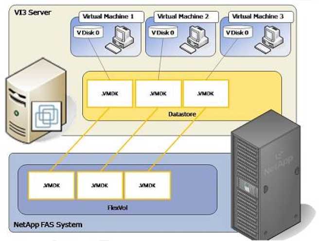
What storage objects make up a virtual machine?

Virtual machines consist of a set of files, and each file has a distinct purpose. Looking at the datastore browser on two virtual machines, you can see these files.

Here is what each of the files is used for:

• vmx the virtual machine configuration file

• vmx. 1ck the virtual machine lock file created when a virtual machine is in a powered-on state. As an example of VMFS locking, it is locked when this file is created, deleted, or modified, but not for the duration of startup/shutdown. Note that the .lck files are not shown in the datastore browser, as they are hidden in the VMFS case, and obscured in the datastore browser itself in the NFS case. In the NFS case, if you mount the NFS datastore directly on another host, you can see the .lck files.

These should not be modified.

• nvram the virtual machine BIOS configuration

• vmdk a virtual machine disk

• -000#. vmdk a virtual machine disk that forms a post-snapshot state when coupled with the base .vmdk

• vmsd the dictionary file for snapshots that couples the base vmdk with the snapshot vmdk

• vmem the virtual machine memory mapped to a file when the virtual machine is in a powered-on state

• vmss the virtual machine suspend file created when a virtual machine is in a suspended state

• -Snapshot#. vmsn the memory state of a virtual machine whose snapshot includes memory state

• vswp the virtual machine swap

Virtual SCSI adapters

Virtual SCSI adapters are what you configure on your virtual machines and attach virtual disks and RDMs to. You can have a maximum of 4 virtual adapters per virtual machine, and each virtual adapter can have 15 devices (virtual disks or RDMs). In the guest, each virtual SCSI adapter has its own HBA queue, so for very intense storage workloads, there are advantages to configuring many virtual SCSI adapters within a single guest. There are several types of virtual adapters in vSphere ESX 4.

Two of these choices are new and are available only if the virtual machines are upgraded to virtual machine 7 (the virtual machine version determines the configuration options, limits and devices of a virtual machine): the LSI Logic SAS virtual SCSI controller (used for W2K8 cluster support) and the VMware paravirtualized SCSI controller, which delivers higher performance.

New vStorage Features in vSphere 4

In this section, we'll cover all the changes and new features in vSphere 4 that are related to storage. Together, these can result in huge efficiency, availability, and performance improvements for most customers.

Some of these include new features inherent to vSphere:

• Thin Provisioning

• VMFS Expansion

• VMFS Resignature Changes

• Hot Virtual Disk Expansion

• Storage VMotion Changes

• Paravirtualized vSCSI

• Improvements to the Software iSCSI Initiator

• Storage Management Improvements

And some of these are new features which focus on integration with third party storage-related functionality:

• VMDirectPath I/O and SR-IOV

• vStorage APIs for Multipathing

• vStorage APIs

Let's take a look at what's new!

Thin Provisioning

The virtual disk behavior in vSphere has changed substantially in vSphere 4, resulting in significantly improved storage efficiency. Most customers can reasonably expect up to a 50 percent higher storage efficiency than with ESX/ESXi 3.5, across all storage types. The changes that result in this dramatic efficiency improvement are as follows:

• The virtual disk format selection is available in the creation CUI, so you can specify type without reverting to vmkfstools command-line options.

• Although vSphere still uses a default format of thick (zeroedthick), for virtual disks created on VMFS datastores (and thin for NFS datastores), in the"Add Hardware" dialog box in the "Create a Disk" step, there's a simple radio button to thin-provision the virtual disk. You should select this if your block storage array doesn't support array-level thin provisioning. If your storage array supports thin provisioning, both thin and thick virtual disk types consume the same amount of actual storage, so you can leave it at the default.

• There is a radio button to configure the virtual disk in advance for the VMware Fault Tolerance (FT) feature which employs the eagerzeroedthick virtual disk format on VMFS volumes, or if the disk will be used in a Microsoft Cluster configuration. Note that in Sphere 4 the virtual disk type can be easily selected via the CUI, including thin provisioning across all array and datastore types. Selecting Support Clustering Features Such As Fault Tolerance creates an eagerzeroedthick virtual disk on VMFS datastores.

Perhaps most important, when using the VMware clone or deploy from template operations, vSphere ESX no longer always uses the eagerzeroedthick format. Rather, when you clone a virtual machine or deploy from a template, a dialog box will appear which enables you to select the destination virtual disk type to thin, thick, or the same type as the source (defaults to the same type as the source). In making the use of VMware-level thin provisioning more broadly applicable, improved reporting on space utilization was needed, and if you examine the virtual machine's Resources tab, you'll see it shows the amount of storage used vs. the amount provisioned. Here, the VM is configured as having a total of 22.78GB of storage (what appears in the VM as available), but only 3.87GB is actually being used on the physical disk.

VMFS Expansion

The VMFS file system can be easily and dynamically expanded in vSphere without adding extents up to the limit of a single volume (2TB-512 bytes), after which continued expansion requires the addition of volumes and VMFS extents. VMFS volumes in vSphere can be expanded up to the 2TB-512 byte limit, and further increases can be achieved using spanned extents.

If the LUN has more capacity than has been configured in the VMFS partition, because most modem storage arrays can nondisruptively add capacity by extending a LUN, it will reflect that in the Expandable column. After clicking Next twice.

VMFS Resignature Changes

Whenever a LUN is presented to an ESX host to be used as a VMFS datastore, it is signed with a VMFS signature. The ESX hosts and vSphere clusters also track the LUNs with an identifier. This identifier was and the LUN identifier was the LUN ID on older ESX 3.x versions and the NAA as of ESX 3.5. Prior to vSphere, when a VMFS volume was presented to an ESX cluster that the cluster had previously or currently accessed (with the same VMFS signature but a different LUN identifier), how the event was handled was relatively complex. Managing the storage device in that case required changing advanced settings such as DisallowSnapshotLUN=O and LVM.EnableResignature=1. This had two problems: the first was that it was a general ESX host setting, not a LUN-specific setting, and so applied universally to all the LUN objects on that ESX host; the second was that it was a little confusing.

Hot Virtual Disk Expansion

Prior to vSphere, extending a virtual disk required that the virtual machine not be running. In vSphere, that ability can be executed while the virtual machine is on. There are a few caveats to extending virtual disks. First, the virtual machine needs to be virtual machine type version 7 (you can upgrade the virtual machine type by right clicking on the virtual machine and selecting "Upgrade Virtual Hardware." Extending a virtual disk that is in the eagerzeroedthick format cannot be done via the CUI whether the virtual machine is on or off.

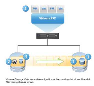
Storage VMotion Changes

Storage VMotion was a feature introduced in VMware Infrastructure 3.5, and it became immediately very popular because it eliminated two of the common causes of planned downtime: moving a virtual machine from one datastore to another; and storage array maintenance or upgrades.

The use cases were broad, and none required that a VM be turned off. Here is a list of key use cases:

• Moving a virtual machine for performance optimization (moving from a slow datastore to a fast datastore, and vice versa)

• Moving a virtual machine for capacity optimization (from a highly utilized datastore to a less utilized datastore)

• For storage tiering (moving noncritical VMs from datastore's on Fibre Channel drives to datastores on SATA drives)

• Wholesale nondisruptive array migration

Some of these use cases are also possible at the array level on various arrays with virtualized storage features. The advantage of doing this at the array or fabric level for both block devices (LUNs) and NAS devices (files) is that the capability can be applied to non-VMware ESX hosts, and that, generally, these virtualized storage capabilities can generally move storage at two to ten times the speed of VMware Storage VMotion. Virtualized storage functionality comes in two types. The first type are cases where the "storage virtualization" is done within the array itself. An example of this type of function is the EMC Virtual LUNs capability. The second type is cases where the "storage virtualization" can be done across multiple arrays also generally in heterogeneous storage environments. Examples of this second type include EMC Invista, EMC Rainfinity, IBM SVC, HDS USP-V, and NetApp vFilers.

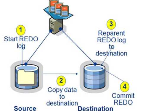
Perhaps more important (but less visible) are the substantial changes under the hood. Understanding these changes requires a short examination on how Storage VMotion worked in VMware Infrastructure 3.5. The image shows the sequence of steps that occur during a Storage VMotion operation in VMware Infrastructure 3.5.

In VMware Infrastructure 3.5,

Storage VMotion starts with the process of an ESX snapshot (step 1), after which the closed VMDK files are copied to the destination (step 2). Then the redo file logs are gradually "reparented" until they are in sync with the source (step 3), at which point they are committed (step 4). The speed of this process is heavily dependent on the performance of the source and destination datastores and on the contention from the workloads in those datastores. However, lGB/minute is achievable, and on large-scale migrations, where Storage VMotion across multiple datastores are used in parallel, +5GB/minute is achievable.

In vSphere, Storage VMotion operates in some substantially improved ways. One of the major changes is the file snapshot-centric mechanism has been changed to a new mechanism: changed block tracking (CBT). It's much faster in general, and it's significantly faster and more reliable during the final stages of the Storage VMotion operation.

During a Storage VMotion operation in vSphere 4, the first step is that all the files except the VMDKs are copied to the new target location.

The second step is that Changed Block Tracking is enabled. The third step is that the bulk of the existing VDMK and vswap files are copied to the new location. During this third step, the changed block locations can be stored on disk or in memory; for most operations, usually memory is used. Subsequently, the baseline blocks are synchronized from the source to the destination-much like with VMotion and then changed blocks. First, these occur in large groups, and then they occur in subsequently smaller and smaller iterations. After they are nearly synchronized, the fourth step occurs, which encompasses a fast suspend/resume interval, which is all that is required to complete the final copy operation. At this point, the virtual machine is running with the virtual disks in the new location. The final, fifth step is when source home and source disks are removed.

This new mechanism is considerably faster than the mechanism used in ESX 3.5 and eliminates the need for the 2x memory requirement needed in 3.5. It should be noted that the primary determinant of Storage VMotion operation speed is still the bandwidth of the source and the destination datastores.

Paravirtualized vSCSI

VMware introduced its first paravirtualized I/O driver in VMware Infrastructure 3.5, with the use of the VMXNET network driver installed when you install VMware Tools. (It has been updated to the third generation, VMXNET3, with the vSphere 4 release.) Paravirtualized guest as drivers communicate more directly with the underlying Virtual Machine Monitor (VMM); they deliver higher throughput and lower latency, and they usually significantly lower the CPU impact of the I/O operations.

In testing, the paravirtualized SCSI driver has shown 30 percent improvements in performance for virtual disks stored on VMFS datastores supported by iSCSI-connected targets, and it has shown between 10 percent and 50 percent improvement for Fiber Channel-connected targets in terms of throughput (lOps) at a given CPU utilization (or lower CPU utilization at a given lOps). In fact, it often delivered half the latency as observed from the guest.

Storage Management Improvements

As VMware environments scale, visualizing the underlying infrastructure becomes more critical for planning and troubleshooting. Also, efficiency starts with having an accurate view of how you're using the assets already deployed. Where is there free capacity? How thin is the thin provisioning?

It's not only a question of efficiency but also availability. Being able to plan the capacity utilization of a system is important for predictive planning and avoiding out-of-space conditions. It's for these reasons that customers use tools, and it's why VMware has a new Storage Views tab with maps and reporting functions in vCenter 4. These native tools represent a small subset of the capabilities, granularity, and visibility, provided by enterprise storage resource management tools that integrate with the vCenter APls under the VMware Ready program, such as EMC Control Center and Storage Scope, Vkemel, Vizoncore, Veeam and others.